Snapshots
How it works
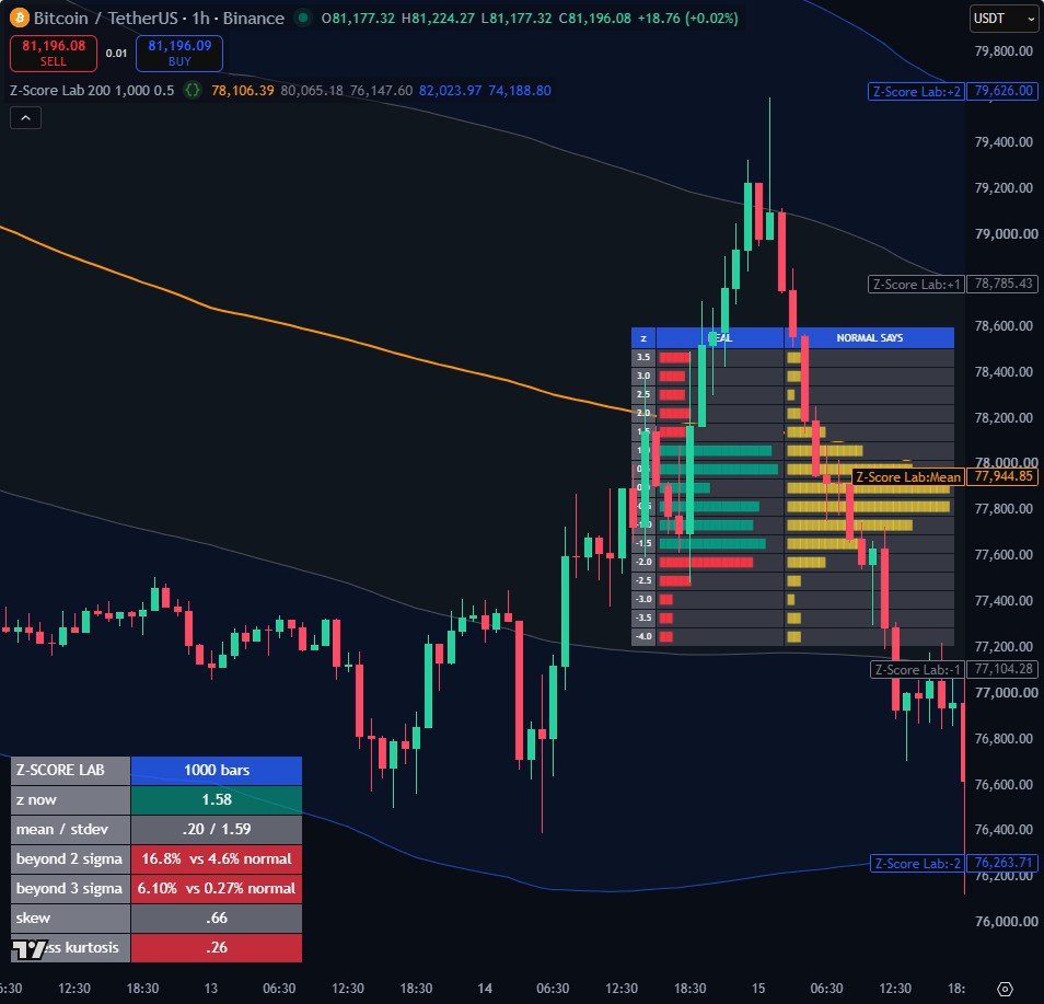
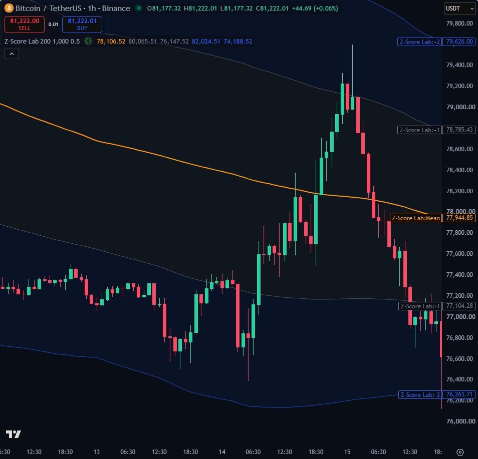
- ta.sma and ta.stdev over the lookback give the mean and the sigma; the z-score is just how many sigmas price sits from that mean.
- The histogram is a table, not a drawing: the z-scores are bucketed into fixed bins and each row is coloured by count, so it renders on any TradingView build.
- The normal comparison uses an Abramowitz-Stegun approximation of the normal CDF, so the expected percentages are computed in Pine rather than hard-coded.
Settings
| Setting | Default | What it does |
|---|---|---|
| Lookback for mean and stdev | 200 | Bars used for the rolling mean and standard deviation |
| Bars in the histogram | 1000 | How much history the z-score histogram counts |
| Histogram bin width (sigma) | 0.5 | Width of each histogram bucket, in sigmas |
| Show what a normal distribution predicts | true | Adds the textbook percentages beside the measured ones |
Source code
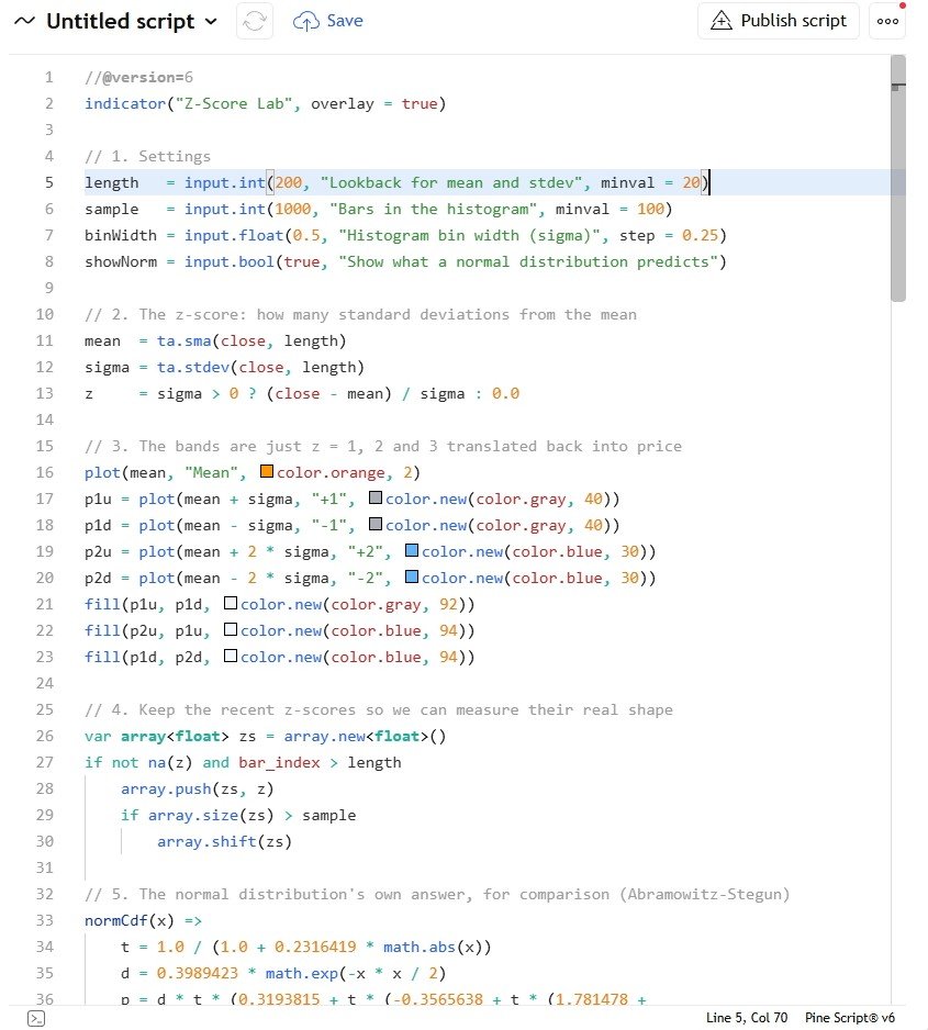
In TradingView: open the Pine Editor, create a new indicator, paste the code, then click "Add to chart".
//@version=6
indicator("Z-Score Lab", overlay = true)

// 1. Settings
length   = input.int(200, "Lookback for mean and stdev", minval = 20)
sample   = input.int(1000, "Bars in the histogram", minval = 100)
binWidth = input.float(0.5, "Histogram bin width (sigma)", step = 0.25)
showNorm = input.bool(true, "Show what a normal distribution predicts")

// 2. The z-score: how many standard deviations from the mean
mean  = ta.sma(close, length)
sigma = ta.stdev(close, length)
z     = sigma > 0 ? (close - mean) / sigma : 0.0

// 3. The bands are just z = 1, 2 and 3 translated back into price
plot(mean, "Mean", color.orange, 2)
p1u = plot(mean + sigma, "+1", color.new(color.gray, 40))
p1d = plot(mean - sigma, "-1", color.new(color.gray, 40))
p2u = plot(mean + 2 * sigma, "+2", color.new(color.blue, 30))
p2d = plot(mean - 2 * sigma, "-2", color.new(color.blue, 30))
fill(p1u, p1d, color.new(color.gray, 92))
fill(p2u, p1u, color.new(color.blue, 94))
fill(p1d, p2d, color.new(color.blue, 94))

// 4. Keep the recent z-scores so we can measure their real shape
var array<float> zs = array.new<float>()
if not na(z) and bar_index > length
    array.push(zs, z)
    if array.size(zs) > sample
        array.shift(zs)

// 5. The normal distribution's own answer, for comparison (Abramowitz-Stegun)
normCdf(x) =>
    t = 1.0 / (1.0 + 0.2316419 * math.abs(x))
    d = 0.3989423 * math.exp(-x * x / 2)
    p = d * t * (0.3193815 + t * (-0.3565638 + t * (1.781478 +
      t * (-1.821256 + t * 1.330274))))
    x > 0 ? 1.0 - p : p

// 6. The stats table and a helper that fills one row
var table t = table.new(position.bottom_left, 2, 7, border_width = 1)
cell(r, a, b, bg) =>
    table.cell(t, 0, r, a, text_color = color.white, bgcolor = color.gray,
      text_size = size.normal, text_halign = text.align_left)
    table.cell(t, 1, r, b, text_color = color.white, bgcolor = bg,
      text_size = size.normal)

// 7. The histogram is drawn as a table too: one row per bin, a bar made of
// block characters. A table is painted by the chart itself, so it stays
// readable at any zoom and never falls off the right-hand edge.
var table h = table.new(position.middle_right, 3, 20, border_width = 1)
blocks(count, pk) =>
    w = int(math.round(26.0 * count / math.max(pk, 1)))
    s = ""
    // a Pine for-loop with a start above its end counts DOWNWARDS,
    // so an empty bin would print two blocks instead of none
    if w > 0
        for i = 1 to w
            s += "█"
    s

// 8. Everything below is measured and drawn once, on the last bar
if barstate.islast and array.size(zs) > 100
    n     = array.size(zs)
    zMean = array.avg(zs)
    zSd   = array.stdev(zs)
    // tail counts: how often price really goes beyond 2 and 3 sigma
    beyond2 = 0
    beyond3 = 0
    m3 = 0.0
    m4 = 0.0
    for i = 0 to n - 1
        v = array.get(zs, i)
        beyond2 += math.abs(v) > 2 ? 1 : 0
        beyond3 += math.abs(v) > 3 ? 1 : 0
        m3 += math.pow(v - zMean, 3)
        m4 += math.pow(v - zMean, 4)
    skew = (m3 / n) / math.pow(zSd, 3)
    kurt = (m4 / n) / math.pow(zSd, 4)

    // 9. Bin the z-scores into a histogram
    bins  = math.round(8 / binWidth)
    counts = array.new_int(bins, 0)
    for i = 0 to n - 1
        v = array.get(zs, i)
        b = math.floor((v + 4) / binWidth)
        b := math.max(0, math.min(bins - 1, b))
        array.set(counts, b, array.get(counts, b) + 1)
    peak = array.max(counts)
    // both columns must share one scale, or the comparison is meaningless
    expPeak = 0.0
    for b = 0 to bins - 1
        e0 = -4 + b * binWidth
        expPeak := math.max(expPeak, n * (normCdf(e0 + binWidth) - normCdf(e0)))
    pk = math.max(peak, expPeak)

    // 10. Print the shape: the real one, and the one the textbook predicts
    table.cell(h, 0, 0, "z", text_color = color.white,
      bgcolor = color.new(color.blue, 20), text_size = size.small)
    table.cell(h, 1, 0, "REAL", text_color = color.white,
      bgcolor = color.new(color.blue, 20), text_size = size.small)
    table.cell(h, 2, 0, showNorm ? "NORMAL SAYS" : "", text_color = color.white,
      bgcolor = color.new(color.blue, 20), text_size = size.small)
    for b = 0 to bins - 1
        zLo = -4 + b * binWidth
        zHi = zLo + binWidth
        c   = array.get(counts, b)
        exp = n * (normCdf(zHi) - normCdf(zLo))
        far = math.abs(zLo) >= 2 or math.abs(zHi) >= 2
        r   = bins - b            // biggest z at the top, like a price axis
        table.cell(h, 0, r, str.tostring(zLo, "#0.0"), text_color = color.white,
          bgcolor = color.new(color.gray, 30), text_size = size.tiny)
        table.cell(h, 1, r, blocks(c, pk),
          text_color = far ? color.red : color.teal,
          bgcolor = color.new(color.black, 0), text_size = size.tiny,
          text_halign = text.align_left)
        table.cell(h, 2, r, showNorm ? blocks(int(exp), pk) : "",
          text_color = color.new(color.yellow, 30),
          bgcolor = color.new(color.black, 0), text_size = size.tiny,
          text_halign = text.align_left)

    // 11. The numbers, so nothing has to be taken on trust
    pct2 = 100.0 * beyond2 / n
    pct3 = 100.0 * beyond3 / n
    cell(0, "Z-SCORE LAB", str.tostring(n) + " bars", color.new(color.blue, 20))
    cell(1, "z now", str.tostring(z, "#.00"),
      math.abs(z) > 2 ? color.new(color.red, 20) : color.new(color.teal, 30))
    cell(2, "mean / stdev", str.tostring(zMean, "#.00") + " / " +
      str.tostring(zSd, "#.00"), color.new(color.gray, 20))
    cell(3, "beyond 2 sigma", str.tostring(pct2, "#.0") + "%  vs 4.6% normal",
      pct2 > 4.6 ? color.new(color.red, 20) : color.new(color.teal, 30))
    cell(4, "beyond 3 sigma", str.tostring(pct3, "#.00") + "%  vs 0.27% normal",
      pct3 > 0.27 ? color.new(color.red, 20) : color.new(color.teal, 30))
    cell(5, "skew", str.tostring(skew, "#.00"), color.new(color.gray, 20))
    cell(6, "excess kurtosis", str.tostring(kurt - 3, "#.00"),
      kurt > 3 ? color.new(color.red, 20) : color.new(color.gray, 20))

// 12. Alert when price is statistically stretched
alertcondition(ta.crossover(z, 2), "Stretched up", "{{ticker}} z above 2")
alertcondition(ta.crossunder(z, -2), "Stretched down", "{{ticker}} z below -2")
Watch it built
This script is written and explained step by step in the video lesson.
Need a custom indicator or strategy?
Non-repainting Pine Script v6, backtested with real costs, alert and webhook ready. Fixed quote within 24 hours.